Randomized Algorithms

• Make random choices during execution
• Traditional algorithms (deterministic algorithms) analyze the behavior of an algorithm on an "average" input, rather than a worst-case input.
• Randomized algorithms do not require new assumptions about the nature of the input. It's purely internal to the algorithm. So it makes the underlying model more powerful.
• 2 broad categories of randomized algorithms
• Las Vegas randomized algorithms
• use randomness to achieve good expected running times, e.g. randomized-quicksort
• guarantee the output is always correct
• Monte Carlo randomized algorithms
• have a deterministic running time
• the output is correct with a certain probability.

Randomized Divide-and-Conquer

the "divide" step is performed using randomization and use expectations of random variables to analyze the time.

Randomized-Selection

• A more general description of finding-the-median problem is selection. Sometimes called Quick-Selection.
• Given a set of n numbers S and a number k between 1 and n, Select(s, k) returns the kth largest element in S.
• Basic Ideas of Select(s, k)
• choose a splitter from s
• partition S into S1 and S2 where {S1} < k and {S2} > k
• if |S1| == k - 1 then splitter is the answer
• if |S1| >= k then answer lies in S1, recursively call Select(s1, k)
• if |S1| < k then answer lies in S2, recursively call Select(s2, k - |S1| - 1)
• Good splitter is very important to make this algorithm running in O(n) time. And should produce each subset into approximately equal in size.
• The deterministic algorithm
• partition the number into n/5 group, so each group has 5 numbers
• find the median of each group, then we have n/5 medians
• recursively find the median from n/5 medians
• use the median as the pivot to partition S into S1 and S2
• recursively search either in S1 or S2
• T(n) = n + T(n/5) + T{max(|S1|, |S2|)} = n + T(n/5) + T(7/10n) => O(n)
• Random Splitters
• choose a "well-centered" splitter = from S uniformly at random
• running time is O(n), the analysis is a little complicated...
• randomized selection (aka quick-selection) is Las Vegas randomized algorithm
• There is a randomized find-approximate-middle algorithm
• pick an element from A uniformly at random (what a simple algorithm!)
• this algorithm returns a correct answer with probability 8/10. It is Monte Carlo randomized algorithm.

Randomized-Quicksort

• improve the Quicksort performance against the worst case instance
• the only difference between randomized-quicksort and deterministic quicksort is in picking on pivot randomness or not to partition the input sequence.
• with randomized picking on pivot, it is expected to have better performance in worst case.
• For instance, with n = 10,000, the probability of X < nln(n) or X > 3nln(n) is less than 0.5%. (data from my instructor's lecture notes.)

Min-cut problem

• Problem description: Given an undirected graph G=(V, E), we define a cut of G to be a partition of V into 2 non-empty sets A and B.
• Deterministic Algorithm for this problem:
• use min-cost s-t cut solution for every pair of vertices
• running time: O(V^5) = (Ford-Fulkerson Algorithm for min-cost s-t cut needs O(V.E) = O(V^3), there are possible V^2 pairs)
• so we can see the power of randomized algorithm.
• Introduce a concept: edge contraction
• pickup any edge (u, v), combine u and v into u'
• remove all edges between u and v
• connect all remaining edges incident to u and v
• Randomized Algorithm of Min-cut (Karger's Algorithm)
• while the graph has more than 2 edges
• randomly pick an edge to contract
• return the remaining edges as min-cut
• running time O(|V|)
• We can test that the algorithm above is not always correct. It is a Monte Carlo randomized algorithm
• Let's look at the probability of correct answer. 
• Say the min-cut edges number is k, the question is how many odd the k edges will survive at last? 
• first, we know the probability of min-cut survive at the first contraction is Pr(min-cut survive) = 1 - k/e   (e is the total number of edges of G)
• observation-1: k <= degrees of every node
• observation-2: (nk/2) <= e    ===> 1 - k/e >= 1 - 2/n = (n-2)/n
• the odds that min-cut survive all n-2 contraction is: <= (n-2)/2 * ((n-1) - 2)/(n-1) * ... * 1/3 = 2/(n(n-1)) = 1/C(n, 2)
• if we execute C(n, 2) runs, the probability of incorrect answer would be: (1 - C(n, 2))^(C(n, 2)) = 1/e = 1/2.7
• as we can see, C(n, 2) runs still seem to result pretty high probability of incorrect answer.
• if we execute ln(n).C(n, 2) runs, the probability of resulting incorrect answer will be 1/n.

Reference

• Algorithm Design, ch13, Kleinberg
• Randomized Algorithm
• Karger's Algorithm

Sorting

Comparison based sorting algorithms

• Bubble sort
• O(n^2), in-place, stable
• Insertion sort
• O(n^2), in-place, stable
• in practical, it is faster for small set of input
• cache friendly
• Selection sort
• O(n^2), in-place, stable
• Merge sort     
• O(nlgn) time, extra space, stable
• This algorithm could be used for big chunk of data which is unable to fit all of them into memory, because we can load part of the data into memory and sort them, at the last, merge each partly sorted pieces.
• Quick sort      
• O(nlgn) time, in-place, constant space, unstable 
• 3 ways to choose pivot
• always pick first one: easy implement but no good performance for sorted input.
• With randomized algorithm running time analysis, which is choosing the pivot number randomly from the input, the worst case running time O(n^2) can be improved to O(nlgn) even for sorted input.
• however, generate random number is not cheap. that comes strategy 3: median-of-3 (left, right, middle) which is more practical and also has good performance.
• Heap sort       
• O(nlgn) time, in-place, stable
• Heap is very good way for extracting max/min although heap sort is a nice application of heap
• BST sort
• O(nlgn) time if we keep the tree balanced

Non-comparison based sorting algorithms

• Counting sort
• has to know the range of input data, for instance, grading could be within 100, age within 200 etc. This is also a limitation of this algorithm.
• need extra linear space to count each element of input
• Bucket sort
• chop data chunk into small pieces, then use other algorithm to sort each piece. In this sense, one could argue it is comparison based sorting algorithm probably.
• assuming the data has uniform distribution, otherwise this method does make much sense.
• divide-and-conquer methodology
• degenerate to counting sort if each element has a bucket
• Radix sort
• sorting based on each digit and put them into queue
• easier way to go through digit from right to left.
• running time: O(kn), k is the digit length of input
• if input has different length of digits, this algorithm also works. Just output those elements with shorter digits, because they were sorted earlier than with longer digits.
• stable

 Why are there so many sorting algorithm?

• depends on size of input (insertion sorting may not that bad for small amount of input, for N <= 20, faster than quicksort)
• depends on data distribution (non-comparison sorting algorithm)
• depends on memory limits (merge sort could be very useful for huge mount of input)

Reference

• Sorting algorithm

Graph - Topological Sort, DFS, BFS

max number of edges:

• n(n-1)/2, for undirected graph
• n(n-1), for directed graph.

Topological Sort

1. only make sense if it is a digraph, and also DAG (Directed Acyclic Graph)
2. there could be more than one topological sort for a graph
3. following is a natural way to get topological sort, besides, we can use DFS to track the finishing order, and it's the reverse order of topological sort.

• ALGORITHM: (O(n + e) + O(n + e) = O(e), e> n generally speaking )
• find the nodes with indegree 0 and put into Q. (O(n + e))
• while Q is not empty
•     n = dequeue(Q)
•     for each edge starts from n, do                      (O(e))
•          n.adj_node.indegree--
•          if (n.adj_node.indgree == 0)  enqueue(Q, n.adj_node)

BFS

1. application of BFS
• testing Bipartite
• Ford-Fulkerson algorithm for maximum flow problem
• Garbage Collection (refer Cheney's algorithm and here)
• detecting cycle (DFS also works)
• path finding (DFS also works)
• Prim's MST and Dijkstra's Single source shortest path use structure similar to BFS.
• find all neighbor nodes in p2p networks, like BitTorrent
• find people within a given distance 'k' from a person in social networking websites

bfs(G, s)         // (O(n + e))
    unmark all vertices
    v = s           // start from here
    do
        if v is marked, continue
        unmark v
        put v.adj_node into Q
        while Q is not empty
            u = dequeue(Q)
            if u is not marked, do
            mark u and enqueue(Q, u)
    while existing unmarked nodes

DFS

1. more broadly used than bfs, since it gives more information
2. differ with BFS which Q, it uses stack to keep the back tracking info
3. two useful thing we can track: the start time and the finishing time, we could do that by just putting its parent node info together into the stack
4. applications
• topological sort is the reverse of finishing time 
• detecting cycle in a graph is another application of dfs
• for unweighted graph, dfs travel produces Minimum Spanning Tree and All-Pair-Shortest-Path.
• find strong connected graph: every vertex is reachable from every vertex.

dfs(G, s)
    mark all vertices as unvisited
    push s into stack S
    while S is not empty
        u = pop(S)
        unmark u
        for all edges (u, v)
            if (v is not visited) push(S, v)

Testing Bipartite (Application of BFS)

Def. An undirected graph G is bipartite if the nodes can be colored blue or white such that every edge has one blue and one white end.

Corollary. A graph is bipartite iff it contains no odd length cycle. That is, no edge between nodes of the same layer, which makes BFS a good application for testing bipartite.

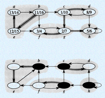
Strongly Connected Components (Application of DFS)

Definition

Given a digraph G=(V, E), a Strongly Connected Components is the subgraph in which any vertex can reach from each other.

Observation

Graph G and its transpose graph have the same Strongly Connected Components. So if vertices u and v are reachable from G iff reachable from its transpose graph.

Algorithm

• DFS(G) computes finishing time for each vertices and produces dfs forest
• GT (transpose G: reverse all edges in G)
• DFS(GT ), but order the vertices in decreasing order of finish time
• the vertices in each DFS tree in the forest of DFS(GT ) is a Strongly Connected Component.
• example (from CLRS book)

• why must do dfs from transpose graph? Consider only nodes {c,d,g} for above graph, if don't dfs to transport graph, and picked up c to do dfs, we get {c,d,g} is a strong connected graph, but it is not.

Reference

• GeeksForGeeks: Application of Breadth First Traversal
• Algorithm Design, ch3, Kleinberg
• Algorithm Theory, Princeton, Spring 2013
• GeeksForGeeks: Ford-Fulkerson Algorithm for Maximum Flow Problem
• Ford-Fulkerson Algorithm

Graph - Minimum Spanning Tree

Spanning Tree

    a spanning tree of an undirected graph is a connected subgraph with no cycles that includes all the vertices

Minimum Spanning Tree

    for undirected edge-weighted graph, MST is a spanning tree with minimum weight.

Two Strategies For Finding MST

• grow the MST from a single vertex, then find a new edge to attach to a single growing tree (Prim's Algorithm)
• maintain a minimum spanning forest, then merge the forest (Kruskal's Algorithm)
• both are greedy algorithm. (pickup a min-cost edge from a single vertex or from the whole graph)

Prim's Algorithm (O(elge) = O(elgn))

• pickup an arbitrary vertex s
• make s as visited
• for all edges (s, u), put (s, u) into min-heap H based on edge cost
• while H is not empty
• e(u, v) = extractMin(H)        // do it e times with O(lge) each time
• mark v as visited                   // u already is marked at this time
• for all edges (v, w)                // do it e times totally
•        if w is unvisited, put (v, w) into H

Kruskal's Algorithm (O(elgn))

• sort all the edges based on their weight. (O(elge) = O(elgn))
• make n different sets. (make_set() * n = O(1 * n))
• for each edges(u, v) in the sorted order
• if (find(u) != find(v))                         // without anything clever, it will take O(n)
• union(find(u), find(v))             // edge(u, v) in the spanning tree. O(1) if found

Union-Find

1. without optimization, running time of Kruskal is: O(elgn) + O(n) + e * O(n)
2. we need to take down the running time of union-find.
3. as a rule of thumb, we should reduce the height of the tree when doing union. 
4. so if we can track the height of a subset, it will be helpful since we can connect the smaller tree to the higher one. it is called "weighted union".
5. with this trick in step 4, find operation could be done in O(lgn). Proof could be done by induction.
6. the cool stuff but hard to proof: if we change a node's parent direct to the root of the set when we do union-find operation each time, the amortized running time could be reduced significantly, but not in constant time. this is called "path compression".
7. path compression does not cost anything, but will give you more benefit in the long run.
8. with the trick like "weighted union" and "path compression", the dominant running time of Kruskal's algorithm is to sort edges, which is O(elgn).
9. Union-Find is easy to implement with data structures like array and others.

Reference

1. https://www.youtube.com/watch?v=ufj5_bppBsA

Hash

Purpose

    To translate an extreme large key space into a reasonably small range of integers.

hashCode = hashFunction(key)

    Typically, maintain a hash table in an array H[0, ..., h-1]
    Handy for the implementation of a dictionary ADT.

Two Issues

• choose hash function - hash code should have uniformed distribution.
• handle collisions - since hash function is many-to-one function.

Hash Functions

• spreads the keys around fairly uniformly (some theoretical work on this subject)
• practice
• choose h as a power of 2
• mod operator can be implemented as: num & (h - 1), because h is a power of 2.
• choose the multiplier a = 8 (h/23) + 5
• hashCode = (a K) mod h    (if K is integer)
• hashCode = (a^2 K1 + aK2) mod h    (if K is a pair of integers)
• hashCode = (a^len*K[1] + a^(len - 1)*K[2] + ... + aK[len]) mod h    (if K is a string)
• double the array size (the hash table) if load factor (n/h) great than 50% (to reduce the probability of collision, typically we choose 2n for the range of hash code). 
• After doubling, should go through the old array and insert the key into the new array using new hash function.
• to reduce the amount of computation, new hash function can be simpler. e.g. hashCode = (2k[1] + 1) for strings.

Collision policies

• Closed address hashing (also called chained hashing) - maintain a linked list for those keys who have the same hash code.
• obviously, the running time for searching in a linked list is O(n)
• why do not use balanced BST? It has theoretical advantages, but it is rarely done in practice. Since load factors are kept small, people more rely on uniformed distributed hash code instead of sophisticated data structures.
• Open address hashing - store all elements on the array of hash table rather than using linked list. 
• more space efficient than closed address hashing.
• searching takes place right in the hash table, so it is likely to be more efficient in time also.
• choose alternative locations is called rehashing.
• the simplest rehashing policy is linear probing, that is, check next available cell until it is not occupied by some other key.
• average cost of a successful search is sqrt(n) which is not a good performance. So why consider this policy? 
• one reason is that the performance is quite good if the load factor is kept low, 50% for example. And with array doubling, it is doable.
• another reason is that a more sophisticated rehashing scheme alleviates the problem of linear probing strategy.
• deletion problem: keys could be cut off from hash table. if we define a constant value as a way to mark "obsolete", then 1) the constant could be reused for a new element. 2) in judging load factor, "obsolete" cells count as elements.
• in conclusion, this strategy of handling collision seems problematic.

Implementation 

• my C code is here.

Reference

• Introduction to design and analysis, 3rd Ed, Sara Baase, section 6.5

Heap

Properties

• order property - key of every node >= the key of its children (for max heap)
• shape property - binary tree and every level completely filled, except the last level which filled from left to right

Operations

• heapify - O(n) (a coarse analysis is O(nlgn), but it's not)
• extractMax - O(lgn)
• insertion - O(lgn)

Others

• a concrete data structure to implement Priority Queue
• designed for finding max / min
• NOT for searching

Application

• Heapsort - O(nlgn) without extra space
• Line segment intersections
• MST (Minimum Spanning Tree) Algorithm (Prim / Kruskal)
• Kth smallest elements - O(n) + O(klgk)

Reference

• Priority Queues
• Heapsort